Introduction and Exproling Raw data

Exploring raw data

Getting a feel for your data

library(readr)
library(dplyr)
library(lubridate)
library(stringr)
library(installr)

Warning message:
"package 'stringr' was built under R version 3.6.3"Warning message:
"package 'installr' was built under R version 3.6.3"
Welcome to installr version 0.22.0

More information is available on the installr project website:
https://github.com/talgalili/installr/

Contact: <tal.galili@gmail.com>
Suggestions and bug-reports can be submitted at: https://github.com/talgalili/installr/issues

            To suppress this message use:
            suppressPackageStartupMessages(library(installr))

weather = readRDS(gzcon(url('https://assets.datacamp.com/production/repositories/34/datasets/b3c1036d9a60a9dfe0f99051d2474a54f76055ea/weather.rds')))

class(weather)

'data.frame'

head(weather)

X	year	month	measure	X1	X2	X3	X4	X5	X6	...	X22	X23	X24	X25	X26	X27	X28	X29	X30	X31
1	2014	12	Max.TemperatureF	64	42	51	43	42	45	...	44	47	46	59	50	52	52	41	30	30
2	2014	12	Mean.TemperatureF	52	38	44	37	34	42	...	39	45	44	52	44	45	46	36	26	25
3	2014	12	Min.TemperatureF	39	33	37	30	26	38	...	33	42	41	44	37	38	40	30	22	20
4	2014	12	Max.Dew.PointF	46	40	49	24	37	45	...	39	45	46	58	31	34	42	26	10	8
5	2014	12	MeanDew.PointF	40	27	42	21	25	40	...	34	42	44	43	29	31	35	20	4	5
6	2014	12	Min.DewpointF	26	17	24	13	12	36	...	25	37	41	29	28	29	27	10	-6	1

tail(weather)

	X	year	month	measure	X1	X2	X3	X4	X5	X6	...	X22	X23	X24	X25	X26	X27	X28	X29	X30	X31
281	281	2015	12	Mean.Wind.SpeedMPH	6	NA	NA	NA	NA	NA	...	NA	NA	NA	NA	NA	NA	NA	NA	NA	NA
282	282	2015	12	Max.Gust.SpeedMPH	17	NA	NA	NA	NA	NA	...	NA	NA	NA	NA	NA	NA	NA	NA	NA	NA
283	283	2015	12	PrecipitationIn	0.14	NA	NA	NA	NA	NA	...	NA	NA	NA	NA	NA	NA	NA	NA	NA	NA
284	284	2015	12	CloudCover	7	NA	NA	NA	NA	NA	...	NA	NA	NA	NA	NA	NA	NA	NA	NA	NA
285	285	2015	12	Events	Rain	NA	NA	NA	NA	NA	...	NA	NA	NA	NA	NA	NA	NA	NA	NA	NA
286	286	2015	12	WindDirDegrees	109	NA	NA	NA	NA	NA	...	NA	NA	NA	NA	NA	NA	NA	NA	NA	NA

str(weather)

'data.frame':   286 obs. of  35 variables:
 $ X      : int  1 2 3 4 5 6 7 8 9 10 ...
 $ year   : int  2014 2014 2014 2014 2014 2014 2014 2014 2014 2014 ...
 $ month  : int  12 12 12 12 12 12 12 12 12 12 ...
 $ measure: chr  "Max.TemperatureF" "Mean.TemperatureF" "Min.TemperatureF" "Max.Dew.PointF" ...
 $ X1     : chr  "64" "52" "39" "46" ...
 $ X2     : chr  "42" "38" "33" "40" ...
 $ X3     : chr  "51" "44" "37" "49" ...
 $ X4     : chr  "43" "37" "30" "24" ...
 $ X5     : chr  "42" "34" "26" "37" ...
 $ X6     : chr  "45" "42" "38" "45" ...
 $ X7     : chr  "38" "30" "21" "36" ...
 $ X8     : chr  "29" "24" "18" "28" ...
 $ X9     : chr  "49" "39" "29" "49" ...
 $ X10    : chr  "48" "43" "38" "45" ...
 $ X11    : chr  "39" "36" "32" "37" ...
 $ X12    : chr  "39" "35" "31" "28" ...
 $ X13    : chr  "42" "37" "32" "28" ...
 $ X14    : chr  "45" "39" "33" "29" ...
 $ X15    : chr  "42" "37" "32" "33" ...
 $ X16    : chr  "44" "40" "35" "42" ...
 $ X17    : chr  "49" "45" "41" "46" ...
 $ X18    : chr  "44" "40" "36" "34" ...
 $ X19    : chr  "37" "33" "29" "25" ...
 $ X20    : chr  "36" "32" "27" "30" ...
 $ X21    : chr  "36" "33" "30" "30" ...
 $ X22    : chr  "44" "39" "33" "39" ...
 $ X23    : chr  "47" "45" "42" "45" ...
 $ X24    : chr  "46" "44" "41" "46" ...
 $ X25    : chr  "59" "52" "44" "58" ...
 $ X26    : chr  "50" "44" "37" "31" ...
 $ X27    : chr  "52" "45" "38" "34" ...
 $ X28    : chr  "52" "46" "40" "42" ...
 $ X29    : chr  "41" "36" "30" "26" ...
 $ X30    : chr  "30" "26" "22" "10" ...
 $ X31    : chr  "30" "25" "20" "8" ...

dim(weather)

1. 286
2. 35

bmi=read_csv('https://assets.datacamp.com/production/repositories/34/datasets/a0a569ebbb34500d11979eba95360125127e6434/bmi_clean.csv')

Parsed with column specification:
cols(
  .default = col_double(),
  Country = col_character()
)
See spec(...) for full column specifications.

class(bmi)

1. 'spec_tbl_df'
2. 'tbl_df'
3. 'tbl'
4. 'data.frame'

dim(bmi)

1. 199
2. 30

head(bmi)

Country	Y1980	Y1981	Y1982	Y1983	Y1984	Y1985	Y1986	Y1987	Y1988	...	Y1999	Y2000	Y2001	Y2002	Y2003	Y2004	Y2005	Y2006	Y2007	Y2008
Afghanistan	21.48678	21.46552	21.45145	21.43822	21.42734	21.41222	21.40132	21.37679	21.34018	...	20.75469	20.69521	20.62643	20.59848	20.58706	20.57759	20.58084	20.58749	20.60246	20.62058
Albania	25.22533	25.23981	25.25636	25.27176	25.27901	25.28669	25.29451	25.30217	25.30450	...	25.46555	25.55835	25.66701	25.77167	25.87274	25.98136	26.08939	26.20867	26.32753	26.44657
Algeria	22.25703	22.34745	22.43647	22.52105	22.60633	22.69501	22.76979	22.84096	22.90644	...	23.69486	23.77659	23.86256	23.95294	24.05243	24.15957	24.27001	24.38270	24.48846	24.59620
Andorra	25.66652	25.70868	25.74681	25.78250	25.81874	25.85236	25.89089	25.93414	25.98477	...	26.75078	26.83179	26.92373	27.02525	27.12481	27.23107	27.32827	27.43588	27.53363	27.63048
Angola	20.94876	20.94371	20.93754	20.93187	20.93569	20.94857	20.96030	20.98025	21.01375	...	21.31954	21.37480	21.43664	21.51765	21.59924	21.69218	21.80564	21.93881	22.08962	22.25083
Antigua and Barbuda	23.31424	23.39054	23.45883	23.53735	23.63584	23.73109	23.83449	23.93649	24.05364	...	24.91721	24.99158	25.05857	25.13039	25.20713	25.29898	25.39965	25.51382	25.64247	25.76602

tail(bmi)

Country	Y1980	Y1981	Y1982	Y1983	Y1984	Y1985	Y1986	Y1987	Y1988	...	Y1999	Y2000	Y2001	Y2002	Y2003	Y2004	Y2005	Y2006	Y2007	Y2008
Venezuela	24.58052	24.69666	24.80082	24.89208	24.98440	25.07104	25.15587	25.24624	25.35274	...	26.50035	26.61021	26.71688	26.79210	26.85498	26.95162	27.05633	27.17698	27.30849	27.44500
Vietnam	19.01394	19.03902	19.06804	19.09675	19.13046	19.16397	19.19740	19.23481	19.27090	...	20.02081	20.10343	20.18623	20.27145	20.36402	20.46585	20.57277	20.68655	20.80189	20.91630
West Bank and Gaza	24.31624	24.40192	24.48713	24.57107	24.65582	24.74148	24.82984	24.91615	25.00108	...	26.28240	26.39074	26.45700	26.48925	26.51152	26.52924	26.54329	26.54449	26.55460	26.57750
Yemen, Rep.	22.90384	22.96813	23.02669	23.07279	23.12566	23.16944	23.20933	23.25043	23.29401	...	23.85482	23.92467	23.99129	24.05692	24.12459	24.19204	24.25638	24.32120	24.37949	24.44157
Zambia	19.66295	19.69512	19.72538	19.75420	19.78070	19.80335	19.82396	19.85065	19.88320	...	20.15094	20.17261	20.20266	20.24298	20.29474	20.35966	20.43398	20.51422	20.59770	20.68321
Zimbabwe	21.46989	21.48867	21.50738	21.52936	21.53383	21.54341	21.54859	21.54590	21.55396	...	21.68873	21.72652	21.76514	21.79645	21.82499	21.85806	21.89495	21.93371	21.97405	22.02660

str(bmi)

tibble [199 x 30] (S3: spec_tbl_df/tbl_df/tbl/data.frame)
 $ Country: chr [1:199] "Afghanistan" "Albania" "Algeria" "Andorra" ...
 $ Y1980  : num [1:199] 21.5 25.2 22.3 25.7 20.9 ...
 $ Y1981  : num [1:199] 21.5 25.2 22.3 25.7 20.9 ...
 $ Y1982  : num [1:199] 21.5 25.3 22.4 25.7 20.9 ...
 $ Y1983  : num [1:199] 21.4 25.3 22.5 25.8 20.9 ...
 $ Y1984  : num [1:199] 21.4 25.3 22.6 25.8 20.9 ...
 $ Y1985  : num [1:199] 21.4 25.3 22.7 25.9 20.9 ...
 $ Y1986  : num [1:199] 21.4 25.3 22.8 25.9 21 ...
 $ Y1987  : num [1:199] 21.4 25.3 22.8 25.9 21 ...
 $ Y1988  : num [1:199] 21.3 25.3 22.9 26 21 ...
 $ Y1989  : num [1:199] 21.3 25.3 23 26 21.1 ...
 $ Y1990  : num [1:199] 21.2 25.3 23 26.1 21.1 ...
 $ Y1991  : num [1:199] 21.2 25.3 23.1 26.2 21.1 ...
 $ Y1992  : num [1:199] 21.1 25.2 23.2 26.2 21.1 ...
 $ Y1993  : num [1:199] 21.1 25.2 23.3 26.3 21.1 ...
 $ Y1994  : num [1:199] 21 25.2 23.3 26.4 21.1 ...
 $ Y1995  : num [1:199] 20.9 25.3 23.4 26.4 21.2 ...
 $ Y1996  : num [1:199] 20.9 25.3 23.5 26.5 21.2 ...
 $ Y1997  : num [1:199] 20.8 25.3 23.5 26.6 21.2 ...
 $ Y1998  : num [1:199] 20.8 25.4 23.6 26.7 21.3 ...
 $ Y1999  : num [1:199] 20.8 25.5 23.7 26.8 21.3 ...
 $ Y2000  : num [1:199] 20.7 25.6 23.8 26.8 21.4 ...
 $ Y2001  : num [1:199] 20.6 25.7 23.9 26.9 21.4 ...
 $ Y2002  : num [1:199] 20.6 25.8 24 27 21.5 ...
 $ Y2003  : num [1:199] 20.6 25.9 24.1 27.1 21.6 ...
 $ Y2004  : num [1:199] 20.6 26 24.2 27.2 21.7 ...
 $ Y2005  : num [1:199] 20.6 26.1 24.3 27.3 21.8 ...
 $ Y2006  : num [1:199] 20.6 26.2 24.4 27.4 21.9 ...
 $ Y2007  : num [1:199] 20.6 26.3 24.5 27.5 22.1 ...
 $ Y2008  : num [1:199] 20.6 26.4 24.6 27.6 22.3 ...
 - attr(*, "spec")=
  .. cols(
  ..   Country = col_character(),
  ..   Y1980 = col_double(),
  ..   Y1981 = col_double(),
  ..   Y1982 = col_double(),
  ..   Y1983 = col_double(),
  ..   Y1984 = col_double(),
  ..   Y1985 = col_double(),
  ..   Y1986 = col_double(),
  ..   Y1987 = col_double(),
  ..   Y1988 = col_double(),
  ..   Y1989 = col_double(),
  ..   Y1990 = col_double(),
  ..   Y1991 = col_double(),
  ..   Y1992 = col_double(),
  ..   Y1993 = col_double(),
  ..   Y1994 = col_double(),
  ..   Y1995 = col_double(),
  ..   Y1996 = col_double(),
  ..   Y1997 = col_double(),
  ..   Y1998 = col_double(),
  ..   Y1999 = col_double(),
  ..   Y2000 = col_double(),
  ..   Y2001 = col_double(),
  ..   Y2002 = col_double(),
  ..   Y2003 = col_double(),
  ..   Y2004 = col_double(),
  ..   Y2005 = col_double(),
  ..   Y2006 = col_double(),
  ..   Y2007 = col_double(),
  ..   Y2008 = col_double()
  .. )

glimpse(bmi)

Rows: 199
Columns: 30
$ Country <chr> "Afghanistan", "Albania", "Algeria", "Andorra", "Angola", "...
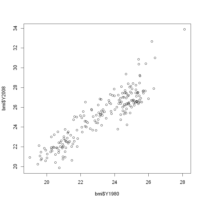
$ Y1980   <dbl> 21.48678, 25.22533, 22.25703, 25.66652, 20.94876, 23.31424,...
$ Y1981   <dbl> 21.46552, 25.23981, 22.34745, 25.70868, 20.94371, 23.39054,...
$ Y1982   <dbl> 21.45145, 25.25636, 22.43647, 25.74681, 20.93754, 23.45883,...
$ Y1983   <dbl> 21.43822, 25.27176, 22.52105, 25.78250, 20.93187, 23.53735,...
$ Y1984   <dbl> 21.42734, 25.27901, 22.60633, 25.81874, 20.93569, 23.63584,...
$ Y1985   <dbl> 21.41222, 25.28669, 22.69501, 25.85236, 20.94857, 23.73109,...
$ Y1986   <dbl> 21.40132, 25.29451, 22.76979, 25.89089, 20.96030, 23.83449,...
$ Y1987   <dbl> 21.37679, 25.30217, 22.84096, 25.93414, 20.98025, 23.93649,...
$ Y1988   <dbl> 21.34018, 25.30450, 22.90644, 25.98477, 21.01375, 24.05364,...
$ Y1989   <dbl> 21.29845, 25.31944, 22.97931, 26.04450, 21.05269, 24.16347,...
$ Y1990   <dbl> 21.24818, 25.32357, 23.04600, 26.10936, 21.09007, 24.26782,...
$ Y1991   <dbl> 21.20269, 25.28452, 23.11333, 26.17912, 21.12136, 24.36568,...
$ Y1992   <dbl> 21.14238, 25.23077, 23.18776, 26.24017, 21.14987, 24.45644,...
$ Y1993   <dbl> 21.06376, 25.21192, 23.25764, 26.30356, 21.13938, 24.54096,...
$ Y1994   <dbl> 20.97987, 25.22115, 23.32273, 26.36793, 21.14186, 24.60945,...
$ Y1995   <dbl> 20.91132, 25.25874, 23.39526, 26.43569, 21.16022, 24.66461,...
$ Y1996   <dbl> 20.85155, 25.31097, 23.46811, 26.50769, 21.19076, 24.72544,...
$ Y1997   <dbl> 20.81307, 25.33988, 23.54160, 26.58255, 21.22621, 24.78714,...
$ Y1998   <dbl> 20.78591, 25.39116, 23.61592, 26.66337, 21.27082, 24.84936,...
$ Y1999   <dbl> 20.75469, 25.46555, 23.69486, 26.75078, 21.31954, 24.91721,...
$ Y2000   <dbl> 20.69521, 25.55835, 23.77659, 26.83179, 21.37480, 24.99158,...
$ Y2001   <dbl> 20.62643, 25.66701, 23.86256, 26.92373, 21.43664, 25.05857,...
$ Y2002   <dbl> 20.59848, 25.77167, 23.95294, 27.02525, 21.51765, 25.13039,...
$ Y2003   <dbl> 20.58706, 25.87274, 24.05243, 27.12481, 21.59924, 25.20713,...
$ Y2004   <dbl> 20.57759, 25.98136, 24.15957, 27.23107, 21.69218, 25.29898,...
$ Y2005   <dbl> 20.58084, 26.08939, 24.27001, 27.32827, 21.80564, 25.39965,...
$ Y2006   <dbl> 20.58749, 26.20867, 24.38270, 27.43588, 21.93881, 25.51382,...
$ Y2007   <dbl> 20.60246, 26.32753, 24.48846, 27.53363, 22.08962, 25.64247,...
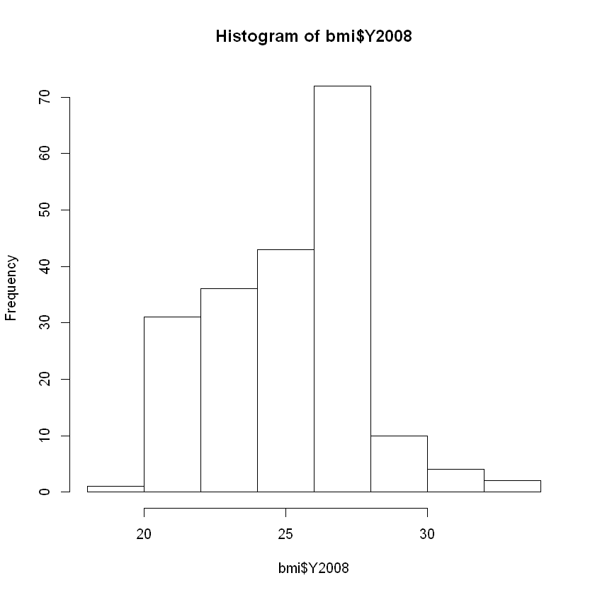
$ Y2008   <dbl> 20.62058, 26.44657, 24.59620, 27.63048, 22.25083, 25.76602,...

# View the first 6 rows
head(bmi, n=6)

# View the first 15 rows
head(bmi, n=15)

# View the last 6 rows
tail(bmi, n=6)

# View the last 10 rows
tail(bmi, n=10)

Country	Y1980	Y1981	Y1982	Y1983	Y1984	Y1985	Y1986	Y1987	Y1988	...	Y1999	Y2000	Y2001	Y2002	Y2003	Y2004	Y2005	Y2006	Y2007	Y2008
Afghanistan	21.48678	21.46552	21.45145	21.43822	21.42734	21.41222	21.40132	21.37679	21.34018	...	20.75469	20.69521	20.62643	20.59848	20.58706	20.57759	20.58084	20.58749	20.60246	20.62058
Albania	25.22533	25.23981	25.25636	25.27176	25.27901	25.28669	25.29451	25.30217	25.30450	...	25.46555	25.55835	25.66701	25.77167	25.87274	25.98136	26.08939	26.20867	26.32753	26.44657
Algeria	22.25703	22.34745	22.43647	22.52105	22.60633	22.69501	22.76979	22.84096	22.90644	...	23.69486	23.77659	23.86256	23.95294	24.05243	24.15957	24.27001	24.38270	24.48846	24.59620
Andorra	25.66652	25.70868	25.74681	25.78250	25.81874	25.85236	25.89089	25.93414	25.98477	...	26.75078	26.83179	26.92373	27.02525	27.12481	27.23107	27.32827	27.43588	27.53363	27.63048
Angola	20.94876	20.94371	20.93754	20.93187	20.93569	20.94857	20.96030	20.98025	21.01375	...	21.31954	21.37480	21.43664	21.51765	21.59924	21.69218	21.80564	21.93881	22.08962	22.25083
Antigua and Barbuda	23.31424	23.39054	23.45883	23.53735	23.63584	23.73109	23.83449	23.93649	24.05364	...	24.91721	24.99158	25.05857	25.13039	25.20713	25.29898	25.39965	25.51382	25.64247	25.76602

Country	Y1980	Y1981	Y1982	Y1983	Y1984	Y1985	Y1986	Y1987	Y1988	...	Y1999	Y2000	Y2001	Y2002	Y2003	Y2004	Y2005	Y2006	Y2007	Y2008
Afghanistan	21.48678	21.46552	21.45145	21.43822	21.42734	21.41222	21.40132	21.37679	21.34018	...	20.75469	20.69521	20.62643	20.59848	20.58706	20.57759	20.58084	20.58749	20.60246	20.62058
Albania	25.22533	25.23981	25.25636	25.27176	25.27901	25.28669	25.29451	25.30217	25.30450	...	25.46555	25.55835	25.66701	25.77167	25.87274	25.98136	26.08939	26.20867	26.32753	26.44657
Algeria	22.25703	22.34745	22.43647	22.52105	22.60633	22.69501	22.76979	22.84096	22.90644	...	23.69486	23.77659	23.86256	23.95294	24.05243	24.15957	24.27001	24.38270	24.48846	24.59620
Andorra	25.66652	25.70868	25.74681	25.78250	25.81874	25.85236	25.89089	25.93414	25.98477	...	26.75078	26.83179	26.92373	27.02525	27.12481	27.23107	27.32827	27.43588	27.53363	27.63048
Angola	20.94876	20.94371	20.93754	20.93187	20.93569	20.94857	20.96030	20.98025	21.01375	...	21.31954	21.37480	21.43664	21.51765	21.59924	21.69218	21.80564	21.93881	22.08962	22.25083
Antigua and Barbuda	23.31424	23.39054	23.45883	23.53735	23.63584	23.73109	23.83449	23.93649	24.05364	...	24.91721	24.99158	25.05857	25.13039	25.20713	25.29898	25.39965	25.51382	25.64247	25.76602
Argentina	25.37913	25.44951	25.50242	25.55644	25.61271	25.66593	25.72364	25.78529	25.84428	...	26.79005	26.88103	26.96067	26.99882	27.04738	27.11001	27.18941	27.28179	27.38889	27.50170
Armenia	23.82469	23.86401	23.91023	23.95649	24.00181	24.04083	24.08736	24.13334	24.17219	...	24.11699	24.18045	24.26670	24.37698	24.50332	24.64178	24.81447	24.99160	25.17590	25.35542
Australia	24.92729	25.00216	25.07660	25.14938	25.22894	25.31849	25.41017	25.50528	25.60001	...	26.65506	26.74486	26.84397	26.93858	27.03801	27.13871	27.24614	27.35267	27.45878	27.56373
Austria	24.84097	24.88110	24.93482	24.98118	25.02208	25.06015	25.10680	25.14747	25.19333	...	25.81773	25.87471	25.93806	25.99583	26.06356	26.14360	26.21107	26.29374	26.38136	26.46741
Azerbaijan	24.49375	24.52584	24.56064	24.60150	24.64121	24.67566	24.71906	24.75799	24.78894	...	24.47842	24.51287	24.57202	24.66021	24.77164	24.89376	25.06256	25.25706	25.45513	25.65117
Bahamas	24.21064	24.30814	24.42750	24.54415	24.66558	24.78408	24.90724	25.03166	25.14778	...	26.12080	26.25748	26.38653	26.51184	26.62607	26.75612	26.88517	27.00715	27.12653	27.24594
Bahrain	23.97588	24.09045	24.20617	24.32335	24.43174	24.53684	24.63328	24.74914	24.86604	...	26.50245	26.65409	26.80388	26.94923	27.09298	27.23908	27.38693	27.53868	27.68865	27.83721
Bangladesh	20.51918	20.47766	20.43741	20.40075	20.36524	20.32983	20.29654	20.26401	20.23497	...	20.13361	20.14774	20.16802	20.18621	20.20948	20.23957	20.27648	20.31554	20.35493	20.39742
Barbados	24.36372	24.43455	24.49314	24.54713	24.59913	24.64998	24.71728	24.77976	24.84265	...	25.51681	25.60292	25.68910	25.77615	25.87020	25.95660	26.06074	26.16874	26.27575	26.38439

Country	Y1980	Y1981	Y1982	Y1983	Y1984	Y1985	Y1986	Y1987	Y1988	...	Y1999	Y2000	Y2001	Y2002	Y2003	Y2004	Y2005	Y2006	Y2007	Y2008
Venezuela	24.58052	24.69666	24.80082	24.89208	24.98440	25.07104	25.15587	25.24624	25.35274	...	26.50035	26.61021	26.71688	26.79210	26.85498	26.95162	27.05633	27.17698	27.30849	27.44500
Vietnam	19.01394	19.03902	19.06804	19.09675	19.13046	19.16397	19.19740	19.23481	19.27090	...	20.02081	20.10343	20.18623	20.27145	20.36402	20.46585	20.57277	20.68655	20.80189	20.91630
West Bank and Gaza	24.31624	24.40192	24.48713	24.57107	24.65582	24.74148	24.82984	24.91615	25.00108	...	26.28240	26.39074	26.45700	26.48925	26.51152	26.52924	26.54329	26.54449	26.55460	26.57750
Yemen, Rep.	22.90384	22.96813	23.02669	23.07279	23.12566	23.16944	23.20933	23.25043	23.29401	...	23.85482	23.92467	23.99129	24.05692	24.12459	24.19204	24.25638	24.32120	24.37949	24.44157
Zambia	19.66295	19.69512	19.72538	19.75420	19.78070	19.80335	19.82396	19.85065	19.88320	...	20.15094	20.17261	20.20266	20.24298	20.29474	20.35966	20.43398	20.51422	20.59770	20.68321
Zimbabwe	21.46989	21.48867	21.50738	21.52936	21.53383	21.54341	21.54859	21.54590	21.55396	...	21.68873	21.72652	21.76514	21.79645	21.82499	21.85806	21.89495	21.93371	21.97405	22.02660

Country	Y1980	Y1981	Y1982	Y1983	Y1984	Y1985	Y1986	Y1987	Y1988	...	Y1999	Y2000	Y2001	Y2002	Y2003	Y2004	Y2005	Y2006	Y2007	Y2008
United States	25.46406	25.57524	25.67883	25.78812	25.90690	26.02568	26.13740	26.25939	26.37687	...	27.60386	27.71039	27.80569	27.90479	28.00041	28.10039	28.19703	28.28959	28.37574	28.45698
Uruguay	24.24001	24.31948	24.39260	24.44209	24.49525	24.54516	24.59804	24.67024	24.73972	...	25.78625	25.86898	25.93469	25.96627	26.00585	26.06073	26.13136	26.20624	26.29256	26.39123
Uzbekistan	24.56500	24.60077	24.62187	24.64780	24.66890	24.69832	24.72305	24.74603	24.77115	...	24.72082	24.75326	24.79418	24.83998	24.88965	24.95455	25.03331	25.12717	25.22226	25.32054
Vanuatu	23.20701	23.32990	23.46016	23.60431	23.75134	23.89466	24.03171	24.15571	24.27529	...	25.72398	25.85208	25.96032	26.05661	26.16060	26.27087	26.38887	26.51376	26.64903	26.78926
Venezuela	24.58052	24.69666	24.80082	24.89208	24.98440	25.07104	25.15587	25.24624	25.35274	...	26.50035	26.61021	26.71688	26.79210	26.85498	26.95162	27.05633	27.17698	27.30849	27.44500
Vietnam	19.01394	19.03902	19.06804	19.09675	19.13046	19.16397	19.19740	19.23481	19.27090	...	20.02081	20.10343	20.18623	20.27145	20.36402	20.46585	20.57277	20.68655	20.80189	20.91630
West Bank and Gaza	24.31624	24.40192	24.48713	24.57107	24.65582	24.74148	24.82984	24.91615	25.00108	...	26.28240	26.39074	26.45700	26.48925	26.51152	26.52924	26.54329	26.54449	26.55460	26.57750
Yemen, Rep.	22.90384	22.96813	23.02669	23.07279	23.12566	23.16944	23.20933	23.25043	23.29401	...	23.85482	23.92467	23.99129	24.05692	24.12459	24.19204	24.25638	24.32120	24.37949	24.44157
Zambia	19.66295	19.69512	19.72538	19.75420	19.78070	19.80335	19.82396	19.85065	19.88320	...	20.15094	20.17261	20.20266	20.24298	20.29474	20.35966	20.43398	20.51422	20.59770	20.68321
Zimbabwe	21.46989	21.48867	21.50738	21.52936	21.53383	21.54341	21.54859	21.54590	21.55396	...	21.68873	21.72652	21.76514	21.79645	21.82499	21.85806	21.89495	21.93371	21.97405	22.02660

Visualizing data

# Histogram of BMIs from 2008
hist(bmi$Y2008)

# Scatter plot comparing BMIs from 1980 to those from 2008
plot(bmi$Y1980, bmi$Y2008)

Tidying data

an overview of the principles of tidy data, how to identify messy data, and what to do about it.

Introduction to tidy data

in bmi, All of the year column names could be expressed as values of a new variable called year.

Gathering columns into key-value pairs

The most important function in tidyr is gather(). It should be used when you have columns that are not variables and you want to collapse them into key-value pairs.

The easiest way to visualize the effect of gather() is that it makes wide datasets long. Running the following command on wide_df will make it long:

gather(wide_df, my_key, my_val, -col)

Spreading key-value pairs into columns

The opposite of gather() is spread(), which takes key-values pairs and spreads them across multiple columns. This is useful when values in a column should actually be column names (i.e. variables). It can also make data more compact and easier to read.

The easiest way to visualize the effect of spread() is that it makes long datasets wide. As you saw in the video, running the following command will make long_df wide:

spread(long_df, my_key, my_val)

Separating columns

The separate() function allows you to separate one column into multiple columns. Unless you tell it otherwise, it will attempt to separate on any character that is not a letter or number. You can also specify a specific separator using the sep argument.

treatments dataset obeys the principles of tidy data, but we’d like to split the treatment dates into two separate columns: year and month. This can be accomplished with the following:

separate(treatments, year_mo, c("year", "month"))

Uniting columns

The opposite of separate() is unite(), which takes multiple columns and pastes them together. By default, the contents of the columns will be separated by underscores in the new column, but this behavior can be altered via the sep argument.

treatments but this time the year_mo column has been separated into year and month. The original column can be recreated by putting year and month back together:

unite(treatments, year_mo, year, month)

Column headers are values, not variable names

You saw earlier, how we sometimes come across datasets where column names are actually values of a variable (e.g. months of the year). This is often the case when working with repeated measures data, where measurements are taken on subjects of interest on multiple occasions over time. The gather() function is helpful in these situations.

Variables are stored in both rows and columns

Sometimes you’ll run into situations where variables are stored in both rows and columns. Although it may not be immediately obvious, if we treat the values in the type column as variables and create a separate column for each of them, we can set things straight. To do this, we use the spread() function.

Multiple values are stored in one column

It’s also fairly common that you will find two variables stored in a single column of data. These variables may be joined by a separator like a dash, underscore, space, or forward slash.

The separate() function comes in handy in these situations. Keep in mind that the into argument, which specifies the names of the 2 new columns being formed, must be given as a character vector (e.g. c("column1", "column2")).

Preparing data for analysis

Type conversions

Loosely speaking, the class() function tells you what type of object you’re working with. (There are subtle differences between the class, type, and mode of an object,

# Make this evaluate to "character"
class(as.character(TRUE))

# Make this evaluate to "numeric"
class(as.numeric("8484.00"))

# Make this evaluate to "integer"
class(as.integer(99L))

# Make this evaluate to "factor"
class(as.factor("factor"))

# Make this evaluate to "logical"
class(as.logical("FALSE"))

'character'

'numeric'

'integer'

'factor'

'logical'

Common type conversions

It is often necessary to change, or coerce, the way that variables in a dataset are stored.

This could be because of the way they were read into R (with read.csv(), for example) or perhaps the function you are using to analyze the data requires variables to be coded a certain way.

Only certain coercions are allowed, but the rules for what works are generally pretty intuitive. For example, trying to convert a character string to a number gives an error: as.numeric("some text").

There are a few less intuitive results. For example, under the hood, the logical values TRUE and FALSE are coded as 1 and 0, respectively. Therefore, as.logical(1) returns TRUE and as.numeric(TRUE) returns 1.

Working with dates

Dates can be a challenge to work with in any programming language, but thanks to the lubridate package, working with dates in R isn’t so bad. Since this project is about cleaning data, we only cover the most basic functions from lubridate to help us standardize the format of dates and times in our data. these functions combine the letters y, m, d, h, m, s, which stand for year, month, day, hour, minute, and second, respectively. The order of the letters in the function should match the order of the date/time you are attempting to read in, although not all combinations are valid. Notice that the functions are “smart” in that they are capable of parsing multiple formats.

students = read_csv('https://assets.datacamp.com/production/repositories/34/datasets/f75a87dbbdf2cf79e2286f97b2af22146cb717b1/students_with_dates.csv')
head(students)

Warning message:
"Missing column names filled in: 'X1' [1]"Parsed with column specification:
cols(
  .default = col_character(),
  X1 = col_double(),
  dob = col_date(format = ""),
  Medu = col_double(),
  Fedu = col_double(),
  traveltime = col_double(),
  studytime = col_double(),
  failures = col_double(),
  famrel = col_double(),
  freetime = col_double(),
  goout = col_double(),
  Dalc = col_double(),
  Walc = col_double(),
  health = col_double(),
  nurse_visit = col_datetime(format = ""),
  absences = col_double()
)
See spec(...) for full column specifications.

X1	school	sex	dob	address	famsize	Pstatus	Medu	Fedu	Mjob	...	romantic	famrel	freetime	goout	Dalc	Walc	health	nurse_visit	absences	Grades
1	GP	F	2000-06-05	U	GT3	A	4	4	at_home	...	no	4	3	4	1	1	3	2014-04-10 14:59:54	6	5/6/6
2	GP	F	1999-11-25	U	GT3	T	1	1	at_home	...	no	5	3	3	1	1	3	2015-03-12 14:59:54	4	5/5/6
3	GP	F	1998-02-02	U	LE3	T	1	1	at_home	...	no	4	3	2	2	3	3	2015-09-21 14:59:54	10	7/8/10
4	GP	F	1997-12-20	U	GT3	T	4	2	health	...	yes	3	2	2	1	1	5	2015-09-03 14:59:54	2	15/14/15
5	GP	F	1998-10-04	U	GT3	T	3	3	other	...	no	4	3	2	1	2	5	2015-04-07 14:59:54	4	6/10/10
6	GP	M	1999-06-16	U	LE3	T	4	3	services	...	no	5	4	2	1	2	5	2013-11-15 14:59:54	10	15/15/15

str(students)

tibble [395 x 33] (S3: spec_tbl_df/tbl_df/tbl/data.frame)
 $ X1         : num [1:395] 1 2 3 4 5 6 7 8 9 10 ...
 $ school     : chr [1:395] "GP" "GP" "GP" "GP" ...
 $ sex        : chr [1:395] "F" "F" "F" "F" ...
 $ dob        : Date[1:395], format: "2000-06-05" "1999-11-25" ...
 $ address    : chr [1:395] "U" "U" "U" "U" ...
 $ famsize    : chr [1:395] "GT3" "GT3" "LE3" "GT3" ...
 $ Pstatus    : chr [1:395] "A" "T" "T" "T" ...
 $ Medu       : num [1:395] 4 1 1 4 3 4 2 4 3 3 ...
 $ Fedu       : num [1:395] 4 1 1 2 3 3 2 4 2 4 ...
 $ Mjob       : chr [1:395] "at_home" "at_home" "at_home" "health" ...
 $ Fjob       : chr [1:395] "teacher" "other" "other" "services" ...
 $ reason     : chr [1:395] "course" "course" "other" "home" ...
 $ guardian   : chr [1:395] "mother" "father" "mother" "mother" ...
 $ traveltime : num [1:395] 2 1 1 1 1 1 1 2 1 1 ...
 $ studytime  : num [1:395] 2 2 2 3 2 2 2 2 2 2 ...
 $ failures   : num [1:395] 0 0 3 0 0 0 0 0 0 0 ...
 $ schoolsup  : chr [1:395] "yes" "no" "yes" "no" ...
 $ famsup     : chr [1:395] "no" "yes" "no" "yes" ...
 $ paid       : chr [1:395] "no" "no" "yes" "yes" ...
 $ activities : chr [1:395] "no" "no" "no" "yes" ...
 $ nursery    : chr [1:395] "yes" "no" "yes" "yes" ...
 $ higher     : chr [1:395] "yes" "yes" "yes" "yes" ...
 $ internet   : chr [1:395] "no" "yes" "yes" "yes" ...
 $ romantic   : chr [1:395] "no" "no" "no" "yes" ...
 $ famrel     : num [1:395] 4 5 4 3 4 5 4 4 4 5 ...
 $ freetime   : num [1:395] 3 3 3 2 3 4 4 1 2 5 ...
 $ goout      : num [1:395] 4 3 2 2 2 2 4 4 2 1 ...
 $ Dalc       : num [1:395] 1 1 2 1 1 1 1 1 1 1 ...
 $ Walc       : num [1:395] 1 1 3 1 2 2 1 1 1 1 ...
 $ health     : num [1:395] 3 3 3 5 5 5 3 1 1 5 ...
 $ nurse_visit: POSIXct[1:395], format: "2014-04-10 14:59:54" "2015-03-12 14:59:54" ...
 $ absences   : num [1:395] 6 4 10 2 4 10 0 6 0 0 ...
 $ Grades     : chr [1:395] "5/6/6" "5/5/6" "7/8/10" "15/14/15" ...
 - attr(*, "spec")=
  .. cols(
  ..   X1 = col_double(),
  ..   school = col_character(),
  ..   sex = col_character(),
  ..   dob = col_date(format = ""),
  ..   address = col_character(),
  ..   famsize = col_character(),
  ..   Pstatus = col_character(),
  ..   Medu = col_double(),
  ..   Fedu = col_double(),
  ..   Mjob = col_character(),
  ..   Fjob = col_character(),
  ..   reason = col_character(),
  ..   guardian = col_character(),
  ..   traveltime = col_double(),
  ..   studytime = col_double(),
  ..   failures = col_double(),
  ..   schoolsup = col_character(),
  ..   famsup = col_character(),
  ..   paid = col_character(),
  ..   activities = col_character(),
  ..   nursery = col_character(),
  ..   higher = col_character(),
  ..   internet = col_character(),
  ..   romantic = col_character(),
  ..   famrel = col_double(),
  ..   freetime = col_double(),
  ..   goout = col_double(),
  ..   Dalc = col_double(),
  ..   Walc = col_double(),
  ..   health = col_double(),
  ..   nurse_visit = col_datetime(format = ""),
  ..   absences = col_double(),
  ..   Grades = col_character()
  .. )

# Coerce Grades to character
students$Grades <- as.character(students$Grades)

# Coerce Medu to factor
students$Medu <- as.factor(students$Medu)

# Coerce Fedu to factor
students$Fedu <- as.factor(students$Fedu)
    
# Look at students once more with str()
str(students)

tibble [395 x 33] (S3: spec_tbl_df/tbl_df/tbl/data.frame)
 $ X1         : num [1:395] 1 2 3 4 5 6 7 8 9 10 ...
 $ school     : chr [1:395] "GP" "GP" "GP" "GP" ...
 $ sex        : chr [1:395] "F" "F" "F" "F" ...
 $ dob        : Date[1:395], format: "2000-06-05" "1999-11-25" ...
 $ address    : chr [1:395] "U" "U" "U" "U" ...
 $ famsize    : chr [1:395] "GT3" "GT3" "LE3" "GT3" ...
 $ Pstatus    : chr [1:395] "A" "T" "T" "T" ...
 $ Medu       : Factor w/ 5 levels "0","1","2","3",..: 5 2 2 5 4 5 3 5 4 4 ...
 $ Fedu       : Factor w/ 5 levels "0","1","2","3",..: 5 2 2 3 4 4 3 5 3 5 ...
 $ Mjob       : chr [1:395] "at_home" "at_home" "at_home" "health" ...
 $ Fjob       : chr [1:395] "teacher" "other" "other" "services" ...
 $ reason     : chr [1:395] "course" "course" "other" "home" ...
 $ guardian   : chr [1:395] "mother" "father" "mother" "mother" ...
 $ traveltime : num [1:395] 2 1 1 1 1 1 1 2 1 1 ...
 $ studytime  : num [1:395] 2 2 2 3 2 2 2 2 2 2 ...
 $ failures   : num [1:395] 0 0 3 0 0 0 0 0 0 0 ...
 $ schoolsup  : chr [1:395] "yes" "no" "yes" "no" ...
 $ famsup     : chr [1:395] "no" "yes" "no" "yes" ...
 $ paid       : chr [1:395] "no" "no" "yes" "yes" ...
 $ activities : chr [1:395] "no" "no" "no" "yes" ...
 $ nursery    : chr [1:395] "yes" "no" "yes" "yes" ...
 $ higher     : chr [1:395] "yes" "yes" "yes" "yes" ...
 $ internet   : chr [1:395] "no" "yes" "yes" "yes" ...
 $ romantic   : chr [1:395] "no" "no" "no" "yes" ...
 $ famrel     : num [1:395] 4 5 4 3 4 5 4 4 4 5 ...
 $ freetime   : num [1:395] 3 3 3 2 3 4 4 1 2 5 ...
 $ goout      : num [1:395] 4 3 2 2 2 2 4 4 2 1 ...
 $ Dalc       : num [1:395] 1 1 2 1 1 1 1 1 1 1 ...
 $ Walc       : num [1:395] 1 1 3 1 2 2 1 1 1 1 ...
 $ health     : num [1:395] 3 3 3 5 5 5 3 1 1 5 ...
 $ nurse_visit: POSIXct[1:395], format: "2014-04-10 14:59:54" "2015-03-12 14:59:54" ...
 $ absences   : num [1:395] 6 4 10 2 4 10 0 6 0 0 ...
 $ Grades     : chr [1:395] "5/6/6" "5/5/6" "7/8/10" "15/14/15" ...
 - attr(*, "spec")=
  .. cols(
  ..   X1 = col_double(),
  ..   school = col_character(),
  ..   sex = col_character(),
  ..   dob = col_date(format = ""),
  ..   address = col_character(),
  ..   famsize = col_character(),
  ..   Pstatus = col_character(),
  ..   Medu = col_double(),
  ..   Fedu = col_double(),
  ..   Mjob = col_character(),
  ..   Fjob = col_character(),
  ..   reason = col_character(),
  ..   guardian = col_character(),
  ..   traveltime = col_double(),
  ..   studytime = col_double(),
  ..   failures = col_double(),
  ..   schoolsup = col_character(),
  ..   famsup = col_character(),
  ..   paid = col_character(),
  ..   activities = col_character(),
  ..   nursery = col_character(),
  ..   higher = col_character(),
  ..   internet = col_character(),
  ..   romantic = col_character(),
  ..   famrel = col_double(),
  ..   freetime = col_double(),
  ..   goout = col_double(),
  ..   Dalc = col_double(),
  ..   Walc = col_double(),
  ..   health = col_double(),
  ..   nurse_visit = col_datetime(format = ""),
  ..   absences = col_double(),
  ..   Grades = col_character()
  .. )

# Preview students2 with str()
str(students)

# Parse as date
dmy("17 Sep 2015")

# Parse as date and time (with no seconds!)
mdy_hm("July 15, 2012 12:56")

# Coerce dob to a date (with no time)
students$dob <- ymd(students$dob)

# Coerce nurse_visit to a date and time
students$nurse_visit <- ymd_hms(students$nurse_visit)
    
# Look at students2 once more with str()
str(students)

tibble [395 x 33] (S3: spec_tbl_df/tbl_df/tbl/data.frame)
 $ X1         : num [1:395] 1 2 3 4 5 6 7 8 9 10 ...
 $ school     : chr [1:395] "GP" "GP" "GP" "GP" ...
 $ sex        : chr [1:395] "F" "F" "F" "F" ...
 $ dob        : Date[1:395], format: "2000-06-05" "1999-11-25" ...
 $ address    : chr [1:395] "U" "U" "U" "U" ...
 $ famsize    : chr [1:395] "GT3" "GT3" "LE3" "GT3" ...
 $ Pstatus    : chr [1:395] "A" "T" "T" "T" ...
 $ Medu       : Factor w/ 5 levels "0","1","2","3",..: 5 2 2 5 4 5 3 5 4 4 ...
 $ Fedu       : Factor w/ 5 levels "0","1","2","3",..: 5 2 2 3 4 4 3 5 3 5 ...
 $ Mjob       : chr [1:395] "at_home" "at_home" "at_home" "health" ...
 $ Fjob       : chr [1:395] "teacher" "other" "other" "services" ...
 $ reason     : chr [1:395] "course" "course" "other" "home" ...
 $ guardian   : chr [1:395] "mother" "father" "mother" "mother" ...
 $ traveltime : num [1:395] 2 1 1 1 1 1 1 2 1 1 ...
 $ studytime  : num [1:395] 2 2 2 3 2 2 2 2 2 2 ...
 $ failures   : num [1:395] 0 0 3 0 0 0 0 0 0 0 ...
 $ schoolsup  : chr [1:395] "yes" "no" "yes" "no" ...
 $ famsup     : chr [1:395] "no" "yes" "no" "yes" ...
 $ paid       : chr [1:395] "no" "no" "yes" "yes" ...
 $ activities : chr [1:395] "no" "no" "no" "yes" ...
 $ nursery    : chr [1:395] "yes" "no" "yes" "yes" ...
 $ higher     : chr [1:395] "yes" "yes" "yes" "yes" ...
 $ internet   : chr [1:395] "no" "yes" "yes" "yes" ...
 $ romantic   : chr [1:395] "no" "no" "no" "yes" ...
 $ famrel     : num [1:395] 4 5 4 3 4 5 4 4 4 5 ...
 $ freetime   : num [1:395] 3 3 3 2 3 4 4 1 2 5 ...
 $ goout      : num [1:395] 4 3 2 2 2 2 4 4 2 1 ...
 $ Dalc       : num [1:395] 1 1 2 1 1 1 1 1 1 1 ...
 $ Walc       : num [1:395] 1 1 3 1 2 2 1 1 1 1 ...
 $ health     : num [1:395] 3 3 3 5 5 5 3 1 1 5 ...
 $ nurse_visit: POSIXct[1:395], format: "2014-04-10 14:59:54" "2015-03-12 14:59:54" ...
 $ absences   : num [1:395] 6 4 10 2 4 10 0 6 0 0 ...
 $ Grades     : chr [1:395] "5/6/6" "5/5/6" "7/8/10" "15/14/15" ...
 - attr(*, "spec")=
  .. cols(
  ..   X1 = col_double(),
  ..   school = col_character(),
  ..   sex = col_character(),
  ..   dob = col_date(format = ""),
  ..   address = col_character(),
  ..   famsize = col_character(),
  ..   Pstatus = col_character(),
  ..   Medu = col_double(),
  ..   Fedu = col_double(),
  ..   Mjob = col_character(),
  ..   Fjob = col_character(),
  ..   reason = col_character(),
  ..   guardian = col_character(),
  ..   traveltime = col_double(),
  ..   studytime = col_double(),
  ..   failures = col_double(),
  ..   schoolsup = col_character(),
  ..   famsup = col_character(),
  ..   paid = col_character(),
  ..   activities = col_character(),
  ..   nursery = col_character(),
  ..   higher = col_character(),
  ..   internet = col_character(),
  ..   romantic = col_character(),
  ..   famrel = col_double(),
  ..   freetime = col_double(),
  ..   goout = col_double(),
  ..   Dalc = col_double(),
  ..   Walc = col_double(),
  ..   health = col_double(),
  ..   nurse_visit = col_datetime(format = ""),
  ..   absences = col_double(),
  ..   Grades = col_character()
  .. )

2015-09-17

[1] "2012-07-15 12:56:00 UTC"

tibble [395 x 33] (S3: spec_tbl_df/tbl_df/tbl/data.frame)
 $ X1         : num [1:395] 1 2 3 4 5 6 7 8 9 10 ...
 $ school     : chr [1:395] "GP" "GP" "GP" "GP" ...
 $ sex        : chr [1:395] "F" "F" "F" "F" ...
 $ dob        : Date[1:395], format: "2000-06-05" "1999-11-25" ...
 $ address    : chr [1:395] "U" "U" "U" "U" ...
 $ famsize    : chr [1:395] "GT3" "GT3" "LE3" "GT3" ...
 $ Pstatus    : chr [1:395] "A" "T" "T" "T" ...
 $ Medu       : Factor w/ 5 levels "0","1","2","3",..: 5 2 2 5 4 5 3 5 4 4 ...
 $ Fedu       : Factor w/ 5 levels "0","1","2","3",..: 5 2 2 3 4 4 3 5 3 5 ...
 $ Mjob       : chr [1:395] "at_home" "at_home" "at_home" "health" ...
 $ Fjob       : chr [1:395] "teacher" "other" "other" "services" ...
 $ reason     : chr [1:395] "course" "course" "other" "home" ...
 $ guardian   : chr [1:395] "mother" "father" "mother" "mother" ...
 $ traveltime : num [1:395] 2 1 1 1 1 1 1 2 1 1 ...
 $ studytime  : num [1:395] 2 2 2 3 2 2 2 2 2 2 ...
 $ failures   : num [1:395] 0 0 3 0 0 0 0 0 0 0 ...
 $ schoolsup  : chr [1:395] "yes" "no" "yes" "no" ...
 $ famsup     : chr [1:395] "no" "yes" "no" "yes" ...
 $ paid       : chr [1:395] "no" "no" "yes" "yes" ...
 $ activities : chr [1:395] "no" "no" "no" "yes" ...
 $ nursery    : chr [1:395] "yes" "no" "yes" "yes" ...
 $ higher     : chr [1:395] "yes" "yes" "yes" "yes" ...
 $ internet   : chr [1:395] "no" "yes" "yes" "yes" ...
 $ romantic   : chr [1:395] "no" "no" "no" "yes" ...
 $ famrel     : num [1:395] 4 5 4 3 4 5 4 4 4 5 ...
 $ freetime   : num [1:395] 3 3 3 2 3 4 4 1 2 5 ...
 $ goout      : num [1:395] 4 3 2 2 2 2 4 4 2 1 ...
 $ Dalc       : num [1:395] 1 1 2 1 1 1 1 1 1 1 ...
 $ Walc       : num [1:395] 1 1 3 1 2 2 1 1 1 1 ...
 $ health     : num [1:395] 3 3 3 5 5 5 3 1 1 5 ...
 $ nurse_visit: POSIXct[1:395], format: "2014-04-10 14:59:54" "2015-03-12 14:59:54" ...
 $ absences   : num [1:395] 6 4 10 2 4 10 0 6 0 0 ...
 $ Grades     : chr [1:395] "5/6/6" "5/5/6" "7/8/10" "15/14/15" ...
 - attr(*, "spec")=
  .. cols(
  ..   X1 = col_double(),
  ..   school = col_character(),
  ..   sex = col_character(),
  ..   dob = col_date(format = ""),
  ..   address = col_character(),
  ..   famsize = col_character(),
  ..   Pstatus = col_character(),
  ..   Medu = col_double(),
  ..   Fedu = col_double(),
  ..   Mjob = col_character(),
  ..   Fjob = col_character(),
  ..   reason = col_character(),
  ..   guardian = col_character(),
  ..   traveltime = col_double(),
  ..   studytime = col_double(),
  ..   failures = col_double(),
  ..   schoolsup = col_character(),
  ..   famsup = col_character(),
  ..   paid = col_character(),
  ..   activities = col_character(),
  ..   nursery = col_character(),
  ..   higher = col_character(),
  ..   internet = col_character(),
  ..   romantic = col_character(),
  ..   famrel = col_double(),
  ..   freetime = col_double(),
  ..   goout = col_double(),
  ..   Dalc = col_double(),
  ..   Walc = col_double(),
  ..   health = col_double(),
  ..   nurse_visit = col_datetime(format = ""),
  ..   absences = col_double(),
  ..   Grades = col_character()
  .. )

String manipulation

Trimming and padding strings

One common issue that comes up when cleaning data is the need to remove leading and/or trailing white space. The str_trim() function from stringr makes it easy to do this while leaving intact the part of the string that you actually want.

> str_trim("  this is a test     ")
[1] "this is a test"

A similar issue is when you need to pad strings to make them a certain number of characters wide. One example is if you had a bunch of employee ID numbers, some of which begin with one or more zeros. When reading these data in, you find that the leading zeros have been dropped somewhere along the way (probably because the variable was thought to be numeric and in that case, leading zeros would be unnecessary.)

> str_pad("24493", width = 7, side = "left", pad = "0")
[1] "0024493"

# Load the stringr package
library(stringr)

# Trim all leading and trailing whitespace
str_trim(c("   Filip ", "Nick  ", " Jonathan"))

# Pad these strings with leading zeros
str_pad(c("23485W", "8823453Q", "994Z"), width=9, side='left', pad='0')

1. 'Filip'
2. 'Nick'
3. 'Jonathan'

1. '00023485W'
2. '08823453Q'
3. '00000994Z'

Examples like this are certainly handy in R. For example, the str_pad() function is useful when importing a dataset with US zip codes. Occasionally R will drop the leading 0 in a zipcode, thinking it’s numeric.

Upper and lower case

In addition to trimming and padding strings, you may need to adjust their case from time to time. Making strings uppercase or lowercase is very straightforward in (base) R thanks to toupper() and tolower(). Each function takes exactly one argument: the character string (or vector/column of strings) to be converted to the desired case.

states <- c("al", "ak", "az", "ar", "ca", "co", "ct", "de", "fl", "ga", "hi", "id", "il", "in", "ia", "ks", "ky", "la", "me", "md", "ma", "mi", "mn", "ms", "mo", "mt", "ne", "nv", "nh", "nj", "nm", "ny", "nc", "nd", "oh", "ok", "or", "pa", "ri", "sc", "sd", "tn", "tx", "ut", "vt", "va", "wa", "wv", "wi", "wy")
# Print state abbreviations
states

# Make states all uppercase and save result to states_upper
states_upper <- toupper(states)
states_upper 

# Make states_upper all lowercase again
tolower(states_upper)

1. 'al'
2. 'ak'
3. 'az'
4. 'ar'
5. 'ca'
6. 'co'
7. 'ct'
8. 'de'
9. 'fl'
10. 'ga'
11. 'hi'
12. 'id'
13. 'il'
14. 'in'
15. 'ia'
16. 'ks'
17. 'ky'
18. 'la'
19. 'me'
20. 'md'
21. 'ma'
22. 'mi'
23. 'mn'
24. 'ms'
25. 'mo'
26. 'mt'
27. 'ne'
28. 'nv'
29. 'nh'
30. 'nj'
31. 'nm'
32. 'ny'
33. 'nc'
34. 'nd'
35. 'oh'
36. 'ok'
37. 'or'
38. 'pa'
39. 'ri'
40. 'sc'
41. 'sd'
42. 'tn'
43. 'tx'
44. 'ut'
45. 'vt'
46. 'va'
47. 'wa'
48. 'wv'
49. 'wi'
50. 'wy'

1. 'AL'
2. 'AK'
3. 'AZ'
4. 'AR'
5. 'CA'
6. 'CO'
7. 'CT'
8. 'DE'
9. 'FL'
10. 'GA'
11. 'HI'
12. 'ID'
13. 'IL'
14. 'IN'
15. 'IA'
16. 'KS'
17. 'KY'
18. 'LA'
19. 'ME'
20. 'MD'
21. 'MA'
22. 'MI'
23. 'MN'
24. 'MS'
25. 'MO'
26. 'MT'
27. 'NE'
28. 'NV'
29. 'NH'
30. 'NJ'
31. 'NM'
32. 'NY'
33. 'NC'
34. 'ND'
35. 'OH'
36. 'OK'
37. 'OR'
38. 'PA'
39. 'RI'
40. 'SC'
41. 'SD'
42. 'TN'
43. 'TX'
44. 'UT'
45. 'VT'
46. 'VA'
47. 'WA'
48. 'WV'
49. 'WI'
50. 'WY'

1. 'al'
2. 'ak'
3. 'az'
4. 'ar'
5. 'ca'
6. 'co'
7. 'ct'
8. 'de'
9. 'fl'
10. 'ga'
11. 'hi'
12. 'id'
13. 'il'
14. 'in'
15. 'ia'
16. 'ks'
17. 'ky'
18. 'la'
19. 'me'
20. 'md'
21. 'ma'
22. 'mi'
23. 'mn'
24. 'ms'
25. 'mo'
26. 'mt'
27. 'ne'
28. 'nv'
29. 'nh'
30. 'nj'
31. 'nm'
32. 'ny'
33. 'nc'
34. 'nd'
35. 'oh'
36. 'ok'
37. 'or'
38. 'pa'
39. 'ri'
40. 'sc'
41. 'sd'
42. 'tn'
43. 'tx'
44. 'ut'
45. 'vt'
46. 'va'
47. 'wa'
48. 'wv'
49. 'wi'
50. 'wy'

Finding and replacing strings

The stringr package provides two functions that are very useful for finding and/or replacing patterns in strings: str_detect() and str_replace().

Like all functions in stringr, the first argument of each is the string of interest. The second argument of each is the pattern of interest. In the case of str_detect(), this is the pattern we are searching for. In the case of str_replace(), this is the pattern we want to replace. Finally, str_replace() has a third argument, which is the string to replace with.

> str_detect(c("banana", "kiwi"), "a")
[1]  TRUE FALSE
> str_replace(c("banana", "kiwi"), "a", "o")
[1] "bonana" "kiwi"

# Copy of students2: students3
students3 <- students

# Look at the head of students3
head(students3)

# Detect all dates of birth (dob) in 1997
str_detect(students3$dob, "1997")

# In the sex column, replace "F" with "Female" ...
students3$sex <- str_replace(students3$sex, "F", "Female")

# ... and "M" with "Male"
students3$sex <- str_replace(students3$sex, "M", "Male")

# View the head of students3
head(students3)

X1	school	sex	dob	address	famsize	Pstatus	Medu	Fedu	Mjob	...	romantic	famrel	freetime	goout	Dalc	Walc	health	nurse_visit	absences	Grades
1	GP	F	2000-06-05	U	GT3	A	4	4	at_home	...	no	4	3	4	1	1	3	2014-04-10 14:59:54	6	5/6/6
2	GP	F	1999-11-25	U	GT3	T	1	1	at_home	...	no	5	3	3	1	1	3	2015-03-12 14:59:54	4	5/5/6
3	GP	F	1998-02-02	U	LE3	T	1	1	at_home	...	no	4	3	2	2	3	3	2015-09-21 14:59:54	10	7/8/10
4	GP	F	1997-12-20	U	GT3	T	4	2	health	...	yes	3	2	2	1	1	5	2015-09-03 14:59:54	2	15/14/15
5	GP	F	1998-10-04	U	GT3	T	3	3	other	...	no	4	3	2	1	2	5	2015-04-07 14:59:54	4	6/10/10
6	GP	M	1999-06-16	U	LE3	T	4	3	services	...	no	5	4	2	1	2	5	2013-11-15 14:59:54	10	15/15/15

1. FALSE
2. FALSE
3. FALSE
4. TRUE
5. FALSE
6. FALSE
7. TRUE
8. FALSE
9. FALSE
10. TRUE
11. FALSE
12. FALSE
13. FALSE
14. TRUE
15. FALSE
16. FALSE
17. TRUE
18. FALSE
19. FALSE
20. FALSE
21. FALSE
22. FALSE
23. TRUE
24. TRUE
25. TRUE
26. FALSE
27. FALSE
28. TRUE
29. FALSE
30. FALSE
31. FALSE
32. FALSE
33. FALSE
34. FALSE
35. TRUE
36. FALSE
37. TRUE
38. FALSE
39. FALSE
40. FALSE
41. FALSE
42. TRUE
43. TRUE
44. FALSE
45. FALSE
46. FALSE
47. TRUE
48. TRUE
49. TRUE
50. TRUE
51. TRUE
52. FALSE
53. FALSE
54. FALSE
55. FALSE
56. FALSE
57. TRUE
58. TRUE
59. FALSE
60. FALSE
61. FALSE
62. FALSE
63. FALSE
64. FALSE
65. FALSE
66. FALSE
67. FALSE
68. TRUE
69. FALSE
70. FALSE
71. TRUE
72. FALSE
73. FALSE
74. FALSE
75. FALSE
76. FALSE
77. FALSE
78. FALSE
79. FALSE
80. FALSE
81. TRUE
82. FALSE
83. FALSE
84. TRUE
85. FALSE
86. FALSE
87. FALSE
88. TRUE
89. FALSE
90. FALSE
91. TRUE
92. TRUE
93. FALSE
94. TRUE
95. FALSE
96. TRUE
97. TRUE
98. FALSE
99. TRUE
100. TRUE
101. FALSE
102. FALSE
103. FALSE
104. FALSE
105. FALSE
106. FALSE
107. FALSE
108. FALSE
109. FALSE
110. FALSE
111. FALSE
112. FALSE
113. FALSE
114. TRUE
115. FALSE
116. TRUE
117. FALSE
118. FALSE
119. FALSE
120. FALSE
121. TRUE
122. TRUE
123. FALSE
124. FALSE
125. FALSE
126. FALSE
127. TRUE
128. FALSE
129. FALSE
130. FALSE
131. FALSE
132. TRUE
133. FALSE
134. FALSE
135. FALSE
136. FALSE
137. TRUE
138. FALSE
139. FALSE
140. FALSE
141. TRUE
142. FALSE
143. FALSE
144. TRUE
145. FALSE
146. TRUE
147. FALSE
148. FALSE
149. TRUE
150. TRUE
151. FALSE
152. FALSE
153. FALSE
154. TRUE
155. FALSE
156. FALSE
157. FALSE
158. FALSE
159. FALSE
160. FALSE
161. FALSE
162. FALSE
163. TRUE
164. FALSE
165. TRUE
166. TRUE
167. TRUE
168. FALSE
169. FALSE
170. FALSE
171. FALSE
172. TRUE
173. TRUE
174. TRUE
175. FALSE
176. FALSE
177. FALSE
178. FALSE
179. FALSE
180. FALSE
181. TRUE
182. FALSE
183. FALSE
184. FALSE
185. FALSE
186. FALSE
187. TRUE
188. FALSE
189. TRUE
190. TRUE
191. TRUE
192. TRUE
193. FALSE
194. FALSE
195. FALSE
196. FALSE
197. FALSE
198. FALSE
199. FALSE
200. FALSE
201. FALSE
202. FALSE
203. FALSE
204. FALSE
205. FALSE
206. FALSE
207. FALSE
208. FALSE
209. FALSE
210. TRUE
211. FALSE
212. FALSE
213. FALSE
214. FALSE
215. FALSE
216. FALSE
217. FALSE
218. TRUE
219. FALSE
220. TRUE
221. FALSE
222. FALSE
223. FALSE
224. FALSE
225. FALSE
226. TRUE
227. TRUE
228. FALSE
229. FALSE
230. FALSE
231. FALSE
232. FALSE
233. FALSE
234. FALSE
235. FALSE
236. FALSE
237. FALSE
238. FALSE
239. TRUE
240. FALSE
241. FALSE
242. FALSE
243. FALSE
244. FALSE
245. FALSE
246. FALSE
247. FALSE
248. FALSE
249. FALSE
250. TRUE
251. FALSE
252. FALSE
253. FALSE
254. FALSE
255. FALSE
256. FALSE
257. FALSE
258. FALSE
259. FALSE
260. FALSE
261. FALSE
262. FALSE
263. FALSE
264. FALSE
265. FALSE
266. FALSE
267. FALSE
268. FALSE
269. FALSE
270. FALSE
271. FALSE
272. FALSE
273. FALSE
274. FALSE
275. FALSE
276. FALSE
277. TRUE
278. FALSE
279. FALSE
280. FALSE
281. FALSE
282. TRUE
283. FALSE
284. TRUE
285. FALSE
286. FALSE
287. FALSE
288. FALSE
289. FALSE
290. FALSE
291. FALSE
292. FALSE
293. FALSE
294. TRUE
295. FALSE
296. FALSE
297. FALSE
298. TRUE
299. FALSE
300. FALSE
301. FALSE
302. FALSE
303. FALSE
304. FALSE
305. FALSE
306. FALSE
307. FALSE
308. FALSE
309. FALSE
310. FALSE
311. FALSE
312. FALSE
313. FALSE
314. FALSE
315. FALSE
316. FALSE
317. FALSE
318. FALSE
319. FALSE
320. FALSE
321. FALSE
322. FALSE
323. FALSE
324. FALSE
325. FALSE
326. FALSE
327. FALSE
328. TRUE
329. FALSE
330. TRUE
331. FALSE
332. FALSE
333. TRUE
334. FALSE
335. FALSE
336. FALSE
337. FALSE
338. FALSE
339. FALSE
340. TRUE
341. FALSE
342. FALSE
343. TRUE
344. FALSE
345. FALSE
346. TRUE
347. FALSE
348. TRUE
349. TRUE
350. FALSE
351. FALSE
352. FALSE
353. FALSE
354. FALSE
355. FALSE
356. FALSE
357. TRUE
358. FALSE
359. FALSE
360. TRUE
361. FALSE
362. TRUE
363. TRUE
364. FALSE
365. FALSE
366. FALSE
367. FALSE
368. FALSE
369. FALSE
370. FALSE
371. FALSE
372. FALSE
373. FALSE
374. TRUE
375. TRUE
376. TRUE
377. FALSE
378. FALSE
379. FALSE
380. FALSE
381. TRUE
382. TRUE
383. TRUE
384. TRUE
385. FALSE
386. FALSE
387. FALSE
388. FALSE
389. FALSE
390. FALSE
391. FALSE
392. FALSE
393. FALSE
394. FALSE
395. FALSE

X1	school	sex	dob	address	famsize	Pstatus	Medu	Fedu	Mjob	...	romantic	famrel	freetime	goout	Dalc	Walc	health	nurse_visit	absences	Grades
1	GP	Female	2000-06-05	U	GT3	A	4	4	at_home	...	no	4	3	4	1	1	3	2014-04-10 14:59:54	6	5/6/6
2	GP	Female	1999-11-25	U	GT3	T	1	1	at_home	...	no	5	3	3	1	1	3	2015-03-12 14:59:54	4	5/5/6
3	GP	Female	1998-02-02	U	LE3	T	1	1	at_home	...	no	4	3	2	2	3	3	2015-09-21 14:59:54	10	7/8/10
4	GP	Female	1997-12-20	U	GT3	T	4	2	health	...	yes	3	2	2	1	1	5	2015-09-03 14:59:54	2	15/14/15
5	GP	Female	1998-10-04	U	GT3	T	3	3	other	...	no	4	3	2	1	2	5	2015-04-07 14:59:54	4	6/10/10
6	GP	Male	1999-06-16	U	LE3	T	4	3	services	...	no	5	4	2	1	2	5	2013-11-15 14:59:54	10	15/15/15

Missing and special values

Finding missing values

social_df = data.frame(name=c('Sarah', 'Tom', 'David', 'Alice'), n_friends=c(244,NA,145,43),status=c('going out', "",'Movie Night', ""))

# Call is.na() on the full social_df to spot all NAs
is.na(social_df)

# Use the any() function to ask whether there are any NAs in the data
any(is.na(social_df))

# View a summary() of the dataset
summary(social_df)

# Call table() on the status column
table(social_df$status)

name	n_friends	status
FALSE	FALSE	FALSE
FALSE	TRUE	FALSE
FALSE	FALSE	FALSE
FALSE	FALSE	FALSE

TRUE

    name     n_friends             status 
 Alice:1   Min.   : 43.0              :2  
 David:1   1st Qu.: 94.0   going out  :1  
 Sarah:1   Median :145.0   Movie Night:1  
 Tom  :1   Mean   :144.0                  
           3rd Qu.:194.5                  
           Max.   :244.0                  
           NA's   :1                      

              going out Movie Night 
          2           1           1 

Dealing with missing values

Missing values can be a rather complex subject, but here we’ll only look at the simple case where you are simply interested in normalizing and/or removing all missing values from your data. For more information on why this is not always the best strategy, search online for “missing not at random.”

Looking at the social_df dataset again, we asked around a bit and figured out what’s causing the missing values that you saw in the last exercise. Tom doesn’t have a social media account on this particular platform, which explains why his number of friends and current status are missing (although coded in two different ways). Alice is on the platform, but is a passive user and never sets her status, hence the reason it’s missing for her.

# Replace all empty strings in status with NA
social_df$status[social_df$status == ""] <- NA

# Print social_df to the console
social_df

# Use complete.cases() to see which rows have no missing values
complete.cases(social_df)

# Use na.omit() to remove all rows with any missing values
na.omit(social_df)

name	n_friends	status
Sarah	244	going out
Tom	NA	NA
David	145	Movie Night
Alice	43	NA

1. TRUE
2. FALSE
3. TRUE
4. FALSE

	name	n_friends	status
1	Sarah	244	going out
3	David	145	Movie Night

Outliers and obvious errors

Dealing with outliers and obvious errors

When dealing with strange values in your data, you often must decide whether they are just extreme or actually erroneous. Extreme values show up all over the place, but you, the data analyst, must figure out when they are plausible and when they are not.

# Look at a summary() of students3
summary(students3)

# View a histogram of the studytime variable
hist(students3$studytime)

# View a histogram of the failures variable
hist(students3$failures)

# View a histogram of absences, but force zeros to be bucketed to the right of zero
hist(students3$failures, right=FALSE)

       X1           school              sex                 dob            
 Min.   :  1.0   Length:395         Length:395         Min.   :1996-11-02  
 1st Qu.: 99.5   Class :character   Class :character   1st Qu.:1997-11-04  
 Median :198.0   Mode  :character   Mode  :character   Median :1998-12-16  
 Mean   :198.0                                         Mean   :1998-10-30  
 3rd Qu.:296.5                                         3rd Qu.:1999-10-29  
 Max.   :395.0                                         Max.   :2000-10-25  
   address            famsize            Pstatus          Medu    Fedu   
 Length:395         Length:395         Length:395         0:  3   0:  2  
 Class :character   Class :character   Class :character   1: 59   1: 82  
 Mode  :character   Mode  :character   Mode  :character   2:103   2:115  
                                                          3: 99   3:100  
                                                          4:131   4: 96  
                                                                         
     Mjob               Fjob              reason            guardian        
 Length:395         Length:395         Length:395         Length:395        
 Class :character   Class :character   Class :character   Class :character  
 Mode  :character   Mode  :character   Mode  :character   Mode  :character  
                                                                            
                                                                            
                                                                            
   traveltime      studytime        failures       schoolsup        
 Min.   :1.000   Min.   :1.000   Min.   :0.0000   Length:395        
 1st Qu.:1.000   1st Qu.:1.000   1st Qu.:0.0000   Class :character  
 Median :1.000   Median :2.000   Median :0.0000   Mode  :character  
 Mean   :1.448   Mean   :2.035   Mean   :0.3342                     
 3rd Qu.:2.000   3rd Qu.:2.000   3rd Qu.:0.0000                     
 Max.   :4.000   Max.   :4.000   Max.   :3.0000                     
    famsup              paid            activities          nursery         
 Length:395         Length:395         Length:395         Length:395        
 Class :character   Class :character   Class :character   Class :character  
 Mode  :character   Mode  :character   Mode  :character   Mode  :character  
                                                                            
                                                                            
                                                                            
    higher            internet           romantic             famrel     
 Length:395         Length:395         Length:395         Min.   :1.000  
 Class :character   Class :character   Class :character   1st Qu.:4.000  
 Mode  :character   Mode  :character   Mode  :character   Median :4.000  
                                                          Mean   :3.944  
                                                          3rd Qu.:5.000  
                                                          Max.   :5.000  
    freetime         goout            Dalc            Walc      
 Min.   :1.000   Min.   :1.000   Min.   :1.000   Min.   :1.000  
 1st Qu.:3.000   1st Qu.:2.000   1st Qu.:1.000   1st Qu.:1.000  
 Median :3.000   Median :3.000   Median :1.000   Median :2.000  
 Mean   :3.235   Mean   :3.109   Mean   :1.481   Mean   :2.291  
 3rd Qu.:4.000   3rd Qu.:4.000   3rd Qu.:2.000   3rd Qu.:3.000  
 Max.   :5.000   Max.   :5.000   Max.   :5.000   Max.   :5.000  
     health       nurse_visit                     absences     
 Min.   :1.000   Min.   :2013-10-28 14:59:54   Min.   : 0.000  
 1st Qu.:3.000   1st Qu.:2014-04-07 02:59:54   1st Qu.: 0.000  
 Median :4.000   Median :2014-09-15 14:59:54   Median : 4.000  
 Mean   :3.554   Mean   :2014-10-10 05:31:11   Mean   : 5.709  
 3rd Qu.:5.000   3rd Qu.:2015-04-08 02:59:54   3rd Qu.: 8.000  
 Max.   :5.000   Max.   :2015-10-15 14:59:54   Max.   :75.000  
    Grades         
 Length:395        
 Class :character  
 Mode  :character  
                   
                   
                   

Another look at strange values

Another useful way of looking at strange values is with boxplots. Simply put, boxplots draw a box around the middle 50% of values for a given variable, with a bolded horizontal line drawn at the median. Values that fall far from the bulk of the data points (i.e. outliers) are denoted by open circles.

boxplot(students3$studytime)